In this post, we’ll explore the fundamental methods used to teach robots new skills. The three main paradigms we’ll explore are:
- Imitation Learning: Teaching robots by showing them what to do
- Reinforcement Learning: Letting robots discover solutions through experience
- Supervised Learning: Using labeled data to build core perception and planning capabilities
Each of these approaches tackles the fundamental challenges of robotic learning in different ways, and modern systems often combine them to leverage their complementary strengths. As part of this post, I have included open-source scripts for a robotic arm that solves a pick-and-place task (similar to our coffee cup examples) using each of the methods discussed. These scripts are available on GitHub at RLFoundations. Due to the natural challenges and computational expense of robotic learning, this repository also includes pre-trained models that can be downloaded from Hugging Face. Please feel free to modify and use them as you see fit, they primarily demonstrate how to implement the IL and model-free RL methods discussed in this post on the simulated robot.
Imitation Learning
Imagine trying to exactly describe to someone how to pickup a coffee cup. Try describing exactly how to pick up the cup, accounting for every finger position, force applied, and possible cup variation. It would be almost impossible, it is far easier to simply show someone how to pick up a coffee cup and have them watch you. This intuition, that some tasks are better shown than described, is the core idea behind Imitation Learning (IL).
The Main Challenge
At first glance, IL may seem straightforward: show the robot what to do, and have it copy those actions. The main problem is even if we demonstrate the task perfectly hundreds of times the robot needs to generalise across various initial conditions, in our coffee cup example this could be:
- Different cup positions and orientations
- Varying lighting conditions
- Different cup sizes, shapes and materials
- Different table heights and surface materials
IL isn’t just about copying demonstrations exactly, it is about extracting the underlying logic that makes the task successful. This generally follows a sequential process of:
- Collect demonstrations
- Learn a mapping from states to actions that captures underlying behaviour
- Handle generalisation by fine-tuning to unseen demonstrations online.
Collecting demonstrations
The first question that arises is how to generate samples that can be used for training, these will generally be task and user specific, some common examples include:
Teleoperation
Teleoperation1 lets operators control robots remotely via VR controllers and joysticks, enabling safe data collection and precise control while protecting operators. However, interface limitations like latency and reduced sensory feedback can restrict the operator’s ability to perform complex manipulations.
Figure 1: NVIDIA Groot, teleoperation of a humanoid robot.
Kinesthetic Demonstrations
Kinesthetic2 teaching enables operators to physically guide robot movements by hand, providing natural and intuitive demonstrations of desired behaviours. While particularly effective for teaching fine-grained manipulation tasks, this method is limited by physical accessibility requirements and operator fatigue.
Figure 2: Wood Planing, kinesthetic programming by demonstration (Alberto Montebelli, Franz Steinmetz and Ville Kyrki Intelligent Robotics - Aalto University, Helsinki).
Third Person Demonstrations
Third-person demonstrations capture human task execution through video recording, allowing efficient collection of natural behavioural data. However, translating actions between human and robot perspectives creates challenges in mapping movements accurately. Ego4D3, Epic Kitchens 4 and Meta’s Project Aria (shown below) are examples of this.
Figure 3: Meta Project Aria (Dima Damen - University of Bristol).
Learning from Demonstrations
Once we have collected a dataset of demonstrations we need to learn a policy from them. Formally given an expert policy $\pi_{E}$ used to generate a dataset of demonstrations $\mathcal{D}={(s_{i},a_{i})}^{N}_{i=1}$, where $s_{i}$ represents states and $a_{i}$ is the experts actions, the objective of IL is to find a policy $\pi$ that approximates $\pi_{E}$, such that:
$$ \pi^* = \arg\min_{\pi} \mathbb{E}_{(s,a) \sim \mathcal{D}} \big[ \mathcal{L}(\pi(a|s), \pi_E(a|s)) \big] $$where $\mathcal{L}$ is a loss function measuring the discrepancy between the learned policy $\pi$ and the expert policy $\pi^{*}$.
Behaviour Cloning5 (BC)
The simplest approach to imitation learning is simply to treat it as a supervised learning problem. Given demonstrations $\tau=(s_{t},a_{t})$, BC directly learns a mapping $\pi_{\theta}(s)\rightarrow a$ by minimising:
$$ \mathcal{L}_{\text{BC}}(\theta) = \mathbb{E}_{(s, a) \sim \tau} [|| \pi_{\theta}(s) - a ||^{2}] $$
Figure 4: BC training process. Demonstrations are initially collected using the oracle $\pi_{E}$ and then trained using supervised learning based on this dataset.
The main problem with pure BC is distributional shift, where small errors accumulate over time as the policy encounters states unseen during training.
Generative Adversarial Imitation Learning6 (GAIL)
GAIL frames IL as a distributional matching problem between policy and expert trajectories using adversarial learning GAIL learns:
- A discriminator $D$ that aims to distinguish between expert and policy generated state-action pairs.
- A policy $\pi$, trained to maximise the discriminator confusion.
GAIL’s optimisation objective is written as:
$$ \min_{\pi} \max_{D} \mathbb{E}_{\pi}[\log(D(s_{t}, a_{t}))]+\mathbb{E}_{\pi_{E}}[\log(1−D(s_{t},a_{t}))]−\lambda H(\pi) $$where $H(\pi)$ is a policy entropy regularization term for exploration.

Figure 5: GAIL training process. The dataset $\mathcal{D}$ is initialized with data from the expert policy $\pi_{E}$, data generated by the adversary is labelled $(s_{t}, a_{t})_{1}$ and $(s_{t}, a_{t})_{0}$ from the policy $\pi_{\theta}$.
Dataset Aggregation7 (DAgger)
DAgger aims to address distributional shift by iteratively collecting corrective demonstrations, this can be written as:
$$ \begin{align*} & \textbf{Initialize: } \text{Train } \pi_1 \text{ on expert demonstrations } \mathcal{D}_0 \\ & \textbf{for } i = 1,2,\dots,N \textbf{ do:} \\ & \quad \text{Execute } \pi_i \text{ to collect states } \{s_1, s_2, \dots, s_n\} \\ & \quad \text{Query expert for labels: } \mathcal{D}_i = \{(s, \pi_{E}(s))\} \\ & \quad \text{Aggregate datasets: } \mathcal{D} = \bigcup_{j=0}^i \mathcal{D}_j \\ & \quad \text{Train } \pi_{i+1} \text{ on } \mathcal{D} \text{ using supervised learning} \\ & \textbf{end for} \end{align*} $$The key problem with DAgger is the need for access to an oracle/expert online to query for expert labels. Variants of Dagger aim to address this and other problems by:
- Selectively querying the expert when confidence is low ThriftyDagger8
- Using filters to prevent the agent executing dangerous actions SafeDAgger9
- Using cost-to-go estimates to improve long-term horizon decision making AggreVaTe10
Reinforcement Learning
While IL relies on demonstrations to teach robots, Reinforcement Learning (RL) takes a fundamentally different yet complementary approach - learning through direct interaction with the environment. Rather than mimicking expert behaviour, RL enables robots to discover optimal solutions through trial and error guided by reward signals.
Problem Definition
RL formalises the learning problem as a Markov Decision Process (MDP), defined by the tuple $(S, A, P, R, \gamma)$ where:
- $S$ is the state space (e.g., joint angles, end-effector pose, visual observations).
- $A$ is the action space (e.g., joint velocities, motor torques).
- $P(s_{t+1}|s_{t},a_{t})$ defines the transition dynamics.
- $R(s_t,a_t)$ provides the reward signal.
- $\gamma \in [0,1]$ is a discount factor for future rewards.
The goal is to learn a policy $\pi(a|s)$ that maximises the expected sum of discounted rewards:
$$ J(\pi)=\mathbb{E}_{\tau \sim \pi} \biggl[ \sum_{t=0}^{\infty} \gamma^{t} R(s_{t},a_{t} ) \biggr] . $$The Main Challenge
Using our coffee cup example, rather than showing the robot how to grasp, we specify a reward signal, perhaps +1 for a successful grasp and 0 otherwise. This seemingly simple shift introduces several key challenges:
Exploration vs Exploitation, a robot learning to grasp cups faces a crucial tradeoff: Should it stick with a mediocre but reliable grasp strategy, or try new motions that could either lead to better grasps or costly failures? Too much exploration risks dropping cups, while too little may prevent discovering optimal solutions.
Credit Assignment, when a grasp succeeds, which specific actions in the trajectory were actually crucial for success? The final gripper closure, the approach vector, or the pre-grasp positioning? The delayed nature of the reward makes it difficult to identify which decisions were truly important.
The Reality Gap between simulation and real-world training. While we can safely attempt millions of grasps in simulation, transferring these policies to physical robots faces numerous challenges:
- Imperfect physics modelling of contact dynamics
- Sensor noise and delays not present in simulation
- Real-world lighting and visual variations
- Physical wear and tear on hardware
These fundamental challenges have driven the development of various RL approaches that we’ll explore in the following sections, from model-based methods that learn explicit world models to hierarchical approaches that break down complex tasks into manageable sub-problems.
Model-Free RL
Model-free methods learn directly from experience, attempting to find optimal policies through trial and error without explicitly modelling how the world works. They can be broadly categorised through three approaches:
1. Value-Based Methods
These approaches learn a value function $Q(s,a)$ that predicts the expected sum of future rewards for taking action $a$ in state $s$. The policy is then derived by selecting actions that maximise this value:
$$ \pi(s) = \arg\max_{a} Q(s,a) . $$The classic example is DQN11, which uses neural networks to approximate Q-values and was initially trained on Breakout. Value-based methods work well in discrete action spaces but struggle with continuous actions common in robotics, as maximising $Q(s,a)$ becomes an expensive optimisation problem.

Figure 6: Deep-Q learning with replay buffer. The agent samples mini-batches from the replay buffer to update the critic network $Q_{\phi}$, while the target network $Q_{\phi}^{T}$ is periodically updated to stabilize the training.
2. Policy Gradient Methods
Rather than learning values, these methods directly optimise a policy $\pi_{\theta}(a|s)$ to maximise expected rewards:
$$ \nabla_{\theta} J(\pi_\theta) = \mathbb{E}_{\tau \sim \pi_\theta} \biggl[ \sum_{t=0}^T \nabla_{\theta} \log \pi_{\theta}(a_{t}|s_{t}) R(\tau) \biggr] $$Policy gradients can naturally handle continuous actions and directly optimise the desired behaviour. However, they often suffer from high variance in gradient estimates, leading to unstable training. This high variance occurs because the algorithm needs to estimate expected returns using a limited number of sampled trajectories, and the correlation between actions and future returns becomes increasingly noisy over long horizons.
Several key innovations have been proposed to address this variance problem:
- Baselines: Subtracting a state-dependent baseline $b(s)$ from returns reduces variance without introducing bias:$$ \nabla_{\theta} J(\pi_\theta) = \mathbb{E}_{\tau \sim \pi_\theta} \biggl[ \sum_{t=0}^T \nabla_{\theta} \log \pi_{\theta}(a_{t}|s_{t}) (R(\tau) - b(s_t)) \biggr].$$
- Advantage estimation12 : Instead of using full returns, we can estimate the advantage $A(s,a) = Q(s,a) - V(s)$ of actions to reduce variance while maintaining unbiased gradients.
- Trust regions13 : TRPO constrains policy updates to prevent destructively large changes by enforcing a KL divergence constraint between old and new policies.
- PPO’s clipped objective14 : Simplifies TRPO by clipping the policy ratio instead of using a hard constraint, providing similar benefits with simpler implementation.
These improvements have made policy gradient methods far more practical for robotic learning, though they still typically require more samples than value-based approaches.

Figure 7: Policy gradient update with replay buffer. The agent stores transition tuples $(s_{t}, a_{t}, r_{t})$ in the buffer and samples mini-batches to update the policy, optimizing actions $a_{t}$ for given state $s_{t}$.
3. Actor-Critic Methods
Actor-critic methods combine the advantages of both approaches:
- An actor (policy) $\pi_\theta(a|s)$ learns to select actions.
- A critic (value function) $Q_\phi(s,a)$ evaluates those actions.
These methods aim to address key limitations of both value-based and policy gradient approaches. Value-based methods struggle with continuous actions common in robotics, while policy gradients suffer from high variance and sample inefficiency. Actor-critic methods tackle these challenges by using the critic to provide lower-variance estimates of expected returns while maintaining the actor’s ability to handle continuous actions.
Soft Actor-Critic15 (SAC) represents the state-of-the-art in this family, and makes use of several key innovations:
- The Maximum Entropy Framework forms the theoretical foundation of SAC, augmenting the standard RL objective with an entropy term. This modification trains the policy to maximise both expected return and entropy simultaneously, automatically trading off exploration vs exploitation. Compared to traditional exploration methods like $\epsilon$-greedy or noise-based approaches, this framework provides greater robustness to hyperparameter choices and enables the discovery of multiple near-optimal behaviors, ultimately leading to better generalization.
- Double Q-Learning with Clipped Critics16, actor-critic methods have a tendency to overestimate the value of the Q-function, leading to suboptimal policies. SAC addresses this by using two Q-functions and taking the minimum of their estimates to reduce overestimation bias and preventing premature convergence.
- The Reparameterisation Trick17 improves policy optimization by making the action sampling process differentiable. The policy network outputs the parameters $(\mu, \sigma)$ from a Gaussian distribution over actions, and actions are sampled from the reparameterisation $a = \mu + \sigma \epsilon$, where $\epsilon \sim \mathcal{N}(0,1)$. This allows for direct backpropagation through the policy network, reducing variance in gradient estimates and improving training stability.
The complete for SAC objective becomes:
$$ J(\pi) = \mathbb{E}_{\tau \sim \pi}\left[\sum_{t=0}^{\infty} \gamma^t (R(s_t,a_t) + \alpha H(\pi(\cdot|s_t)))\right] $$where $H(\pi(\cdot|s_t))$ is the entropy of the policy and $\alpha$ balances exploration with exploitation.

Figure 8: Actor-Critic update with Advantage Estimation and replay buffer. The actor $\pi_{\theta}$ updates its policy using the advantage estimate, $A^{\pi}(s_{t}, a_{t}) = Q^{\pi}(s_{t}, a_{t}) - V^{\pi}(s_{t})$. The target network $Q_{\phi}^{T}$ stabilizes learning by providing periodic updates to the critic.
SAC has become the preferred choice for robotic learning18 because it:
- Learns efficiently from off-policy data
- Automatically adjusts exploration through entropy maximisation
- Provides stable training across different hyperparameter settings
- Achieves state-of-the-art sample efficiency and asymptotic performance
Model-Based RL (MBRL)
Model-based RL aims to improve sample efficiency by learning a dynamics model of the environment and using it for planning or policy learning. The key idea is that if we can predict how our actions affect the world, we can learn more efficiently from limited real-world data.
The core idea of MBRL can be broken down into three key components:
- Data Collection: interact with the environment to collect trajectories
- Model Learning: Train a dynamics model to predict state transitions
- Policy Optimisation: Use the model to improve the policy through planning or simulation
Ideally this begins a cycle where better models lead to be to better policies, which in turn collect better data.
Learning the Dynamics Model
Given collected transitions we need to learn a function $f_\theta$ that predicts how our actions change the world:
$$ \hat{s}_{t+1} = f_\theta(s_t, a_t) \approx P(s_{t+1}|s_t,a_t) $$For robotic tasks, this model can take two forms:
Deterministic Models: Directly predict the next state, like if I close the gripper by 2cm, the cup will move up by 5cm.
Probabilistic Models: Capture uncertainty in predictions:
$$ P(s_{t+1}∣s_{t},a_{t})=\mathcal{N} \bigl( \mu_{\theta}(s_{t},a_{t}),\Sigma_{\theta}(s_{t},a_{t}) \bigr) $$For example, predicting closing the gripper has a 90% chance of stable grasp, 10% chance of knocking the cup over. This type of modelling has proven to be useful for safe learning.
Once we have a dynamics model, there are two fundamentally different approaches:
Planning-Based Control
Planning methods use the model to simulate and evaluate potential future trajectories. The two main approaches are:
Model Predictive Control19 (MPC) repeatedly solves a finite-horizon optimisation problem at each time-step:
$$ a_{t:t+H}=\arg\max_{a_{t:t+H}} \sum_{h=0}^{H} r(s_{h},a_{h}) \ \text{where} \ s_{h+1}=f_{\theta}(s_{h},a_{h}) $$This optimisation problem is often solved using a sampling-based approaches like Cross-Entropy Method (CEM) or Covariance Matrix Adaptation Evolution Strategy (CMA-ES) which are often favored because they are easily parallelisable on GPUs and can optimise nonlinear, high-dimensional action spaces without requiring derivatives of the cost function. These methods iteratively sample and refine candidate action sequences, making them well-suited for complex control tasks. The general MPC process at each time step $t$ is:
- Generate $K$ action sequences: $$\{a_{t:t+H}^{(k)}\}_{k=1}^{K}$$
- Simulate trajectories using model: $s_{h+1}^{(k)} = f_{\theta}(s_h^{(k)}, a_h^{(k)})$.
- Execute first action of the best sequence: $$ a_t = a_{t:t+H}^{(k)}[0]$$ where $$k^{*} = \arg\max_k \sum_{h=0}^{H} r(s_h^{(k)}, a_h^{(k)}).$$
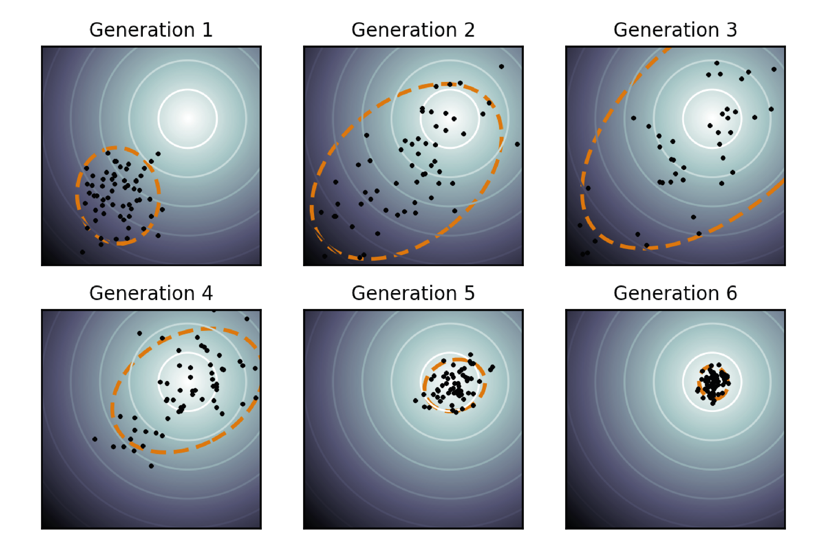
Figure 9: Covariance Matrix Adaptation Evolution Strategy (CMA-ES). Black dots represent sampled candidate solutions, while the orange ellipses illustrate the evolving covariance matrix. The algorithm progressively refines its distribution toward the global minima as variance reduces.
Gradient-Based Planning methods use the differentiability of both the learned dynamics model $f_{\theta}$ and the reward function $r(s_{h}, a_{h})$ to compute the gradient of the expected return with respect to the action sequence $a_{t:t+H}$, enabling direct optimisation through gradient descent. Compared to sampling based methods by following the gradient of expected return the planner can rapidly converge to high-value action sequences without extensive random sampling. This is both more computationally efficient precise than sampling based methods. As the continuous optimisation space offers results in more accurate actions for fine control outputs.
Methods like PETS20 optimise action sequences directly through gradient descent on the expected return:
$$ J(a_{t:t+H}) = \mathbb{E}_{s_{h+1} \sim f_{\theta}(s_{h}, a_{h}}) \biggl[ \sum_{h=0}^{H} r(s_{h}, a_{h}) \biggr] $$ $$ a_{t:t+H}^{*} = \arg \max_{a_{t:t+H}} J(a_{t:t+H}) $$Building on this Dreamer extends gradient-based planning to latent space, where it learns a world model that can be efficiently differentiated through time. By planning in a learned latent space, rather than raw observations, Dreamer can handle high-dimensional inputs whilst maintaining the computational benefits of gradient-based optimisation.
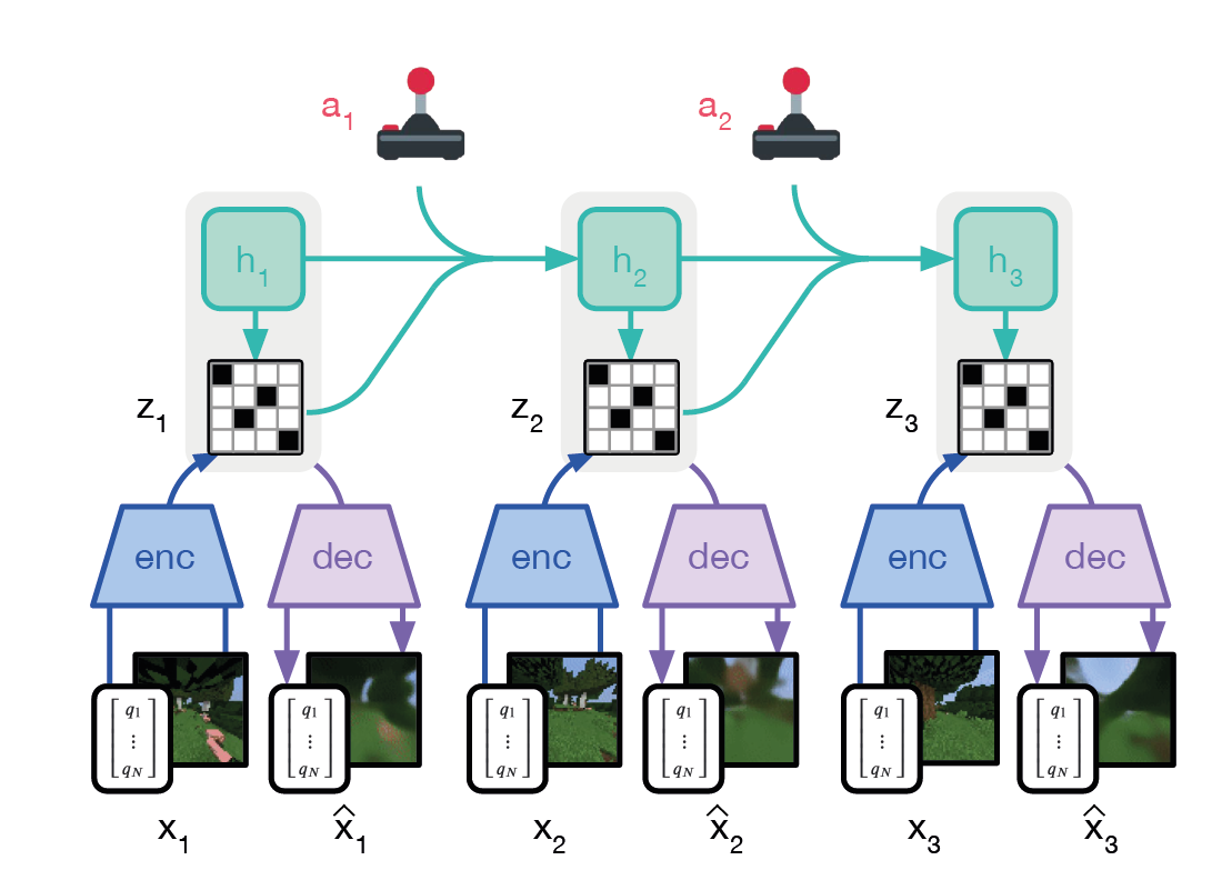
Figure 10: Dreamer recurrent world model with an encoder-decoder structure. The model predicts latent states $z_{t}$ from observations $x_{t}$, generating reconstructions $\hat{x}_{t}$. The recurrent module $h_{t}$ captures temporal dependencies, while the model uses latent dynamics to predict future states and inform actions $a_{t}$.
The main problem with all of these methods is how they deal with non-differentiable dynamics or discontinuous rewards, which can lead to sparse optima or unstable gradients. These problems can be addressed with methods like smoothing functions or robust optimisation, but this naturally adds more engineering effort and can harm performance.
Model-Based Policy Learning
Rather than planning actions online, an alternative approach is to leverage the learned dynamics model to train a policy through simulated experiences. This approach combines the sample efficiency of model-based methods with the fast inference of model-free policies.
Dynastyle Algorithms21 mix real and simulated data for policy updates. By mixing experiences from both sources, these methods balance the bias-variance trade-off between potentially imperfect model predictions and limited real-world data. This objective becomes:
$$ J( \pi_{\phi}) = \alpha \mathbb{E}_{(s, a) \sim \mathcal{D}_{\text{real}}} [Q(s, a)] + (1-\alpha)\mathbb{E}_{(s, a) \sim \mathcal{D}_{\text{model}}} [Q(s, a)] $$where $\mathcal{D}_{\text{real}}$ is collected from the real environment and $\mathcal{D}_{\text{model}}$ is generated using the learned model $f_{\theta}$. The mixing coefficient $\alpha$ controls the trade-off between real and simulated data.
Model Based Policy Optimisation22 (MBPO) addresses the challenge of compounding prediction errors in learned dynamics models by limiting synthetic rollouts to short horizons. The main insight is that although learned models become unreliable for long-term predictions, they remain accurate for short-term forecasting, making them valuable for generating high-quality synthetic data. To ensure reliability MBPO incorporates two mechanisms to handle two types of uncertainty:
- Aleatoric Uncertainty is randomness inherent to the enviornment that cannot be reduced by collecting larger quantitys of data. To account for this MBPO models transitions as probabilistic distributions rather than fixed outcomes. Each network outputs a Gaussian distribution over possible next states:
- Epistemic Uncertainty, is uncertainty in the model itself and comes from limited or biased training data and can be reduced with better model learning. MBPO handles epistemic uncertainty via an ensemble of models $(p_\theta^1,…,p_\theta^B)$. During synthetic rollouts, one model is randomly selected for each prediction. This approach ensures that predictions reflect the range of plausible dynamics, avoiding overconfidence in poorly understood regions of the state space.
The algorithm can be summarized as follows:
$$ \begin{align*} & \textbf{Initialize: } \text{Policy: } \pi_\phi, \text{ Model Ensemble: } \{p_\theta^1,...,p_\theta^B\}, \text{ Replay Buffers: } \{ \mathcal{D}_\text{env}, \mathcal{D}_{\text{model}} \} \\ & \textbf{for } N \text{ epochs do:} \\ & \quad \text{for } E \text{ steps do:} \\ & \quad \quad \text{Take action in environment: } a_t \sim \pi_\phi(s_t) \\ & \quad \quad \text{Add to replay buffer: } \mathcal{D}_\text{env} \leftarrow \mathcal{D}_\text{env} \cup \{(s_t, a_t, r_t, s_{t+1})\} \\ & \quad \text{for } i = 1,\dots,B \text{ do:} \\ & \quad \quad \text{Train } p_\theta^i \text{ on bootstrapped sample from } \mathcal{D}_\text{env} \\ & \quad \text{for } M \text{ model rollouts do:} \\ & \quad \quad s_t \sim \mathcal{D}_\text{env} \text{ // Sample real state} \\ & \quad \quad \text{for } k = 1,\dots,K \text{ steps do:} \\ & \quad \quad \quad a_{t+k} \sim \pi_\phi(s_{t+k}) \\ & \quad \quad \quad i \sim \text{Uniform}(1,B) \text{ // Sample model from ensemble} \\ & \quad \quad \quad s_{t+k+1} \sim p_\theta^i(s_{t+k+1}|s_{t+k}, a_{t+k}) \\ & \quad \quad \quad \mathcal{D}_\text{model} \leftarrow \mathcal{D}_\text{model} \cup \{(s_{t+k}, a_{t+k}, r_{t+k}, s_{t+k+1})\} \\ & \quad \text{for } G \text{ gradient updates do:} \\ & \quad \quad \phi \leftarrow \phi - \lambda_\pi \nabla_\phi J_\pi(\phi, \mathcal{D}_\text{model}) \\ & \textbf{end for} \end{align*} $$Where:
- $K$ is the model rollout horizon
- $f_\theta$ is an ensemble of probabilistic neural networks
- $J_\pi$ is the policy optimization objective (often SAC)
- $\lambda_\pi$ is the learning rate
In practice, MBPO has proven particularly effective for robotic control tasks, where collecting real-world data is expensive.
Challenges in MBRL
MBRL faces several fundamental challenges that make it particularly difficult in robotics:
Compounding Model Errors, are a significant problem in MBRL. A small error in predicting finger position at $t=1$ results in slightly incorrect contact points, which leads to larger errors in predicted contact forces at $t=2$. By $t=10$, the model might predict a successful grasp while in reality the cup has been knocked over. This error accumulation can be expressed formally, given a learned model $f_{\theta}$, this prediction error grows approximately exponentially with horizon $H$:
$$||\hat{s}_{H} - s_{H}|| \approx \|\nabla f_{\theta}\|^H \|\epsilon\|$$where $\epsilon$ is the one-step prediction error.
Real-World Physics presents significant challenges due to its discontinuous nature, especially during object interactions and contacts. Learned models struggle to capture these discontinuities because they must simultaneously handle two distinct regimes: continuous dynamics in free space and discontinuous dynamics during contact. Additionally, the system exhibits high sensitivity to initial conditions, where microscopic variations in parameters like surface friction can lead to macroscopically different outcomes, for instance, determining whether a gripper maintains or loses its grasp on an object. These abrupt transitions between physical states and the sensitive dependence on initial conditions make it particularly challenging to learn and maintain accurate predictive models.
Supervised Learning
A key question in designing robotic systems is whether to pursue an end-to-end approach that learns directly from raw sensory inputs to actions, or decompose the problem into modular components that can be trained independently. End-to-end learning offers the theoretical advantage of learning optimal task-specific representations and avoiding hand-engineered decompositions. The main idea is that by training the entire perception-to-action pipeline jointly, the system can learn representations that are optimally suited for the task.
Whilst appealing in theory, end-to-end learning faces several practical challenges in real robotics. End-to-end systems typically require vast quantities of task-specific data, as they must learn everything from scratch for each new task. They also tend to be brittle, a change in lighting conditions or robot configuration might require retraining the entire system. But perhaps the most significant challenge is the lack of interpretability, end-to-end systems are often described as black boxes because it is difficult to understand how they arrive at their decisions. This makes it hard to diagnose failures or understand why the system behaves in a particular way.
In contrast, modular approaches break down the robotic learning problem into specialized components - typically perception, state estimation, planning, and control. Each module can be trained independently using techniques best suited for its specific challenges. This decomposition offers several key advantages:
- Interpretability: Each module can be understood and debugged independently, making it easier to diagnose failures and understand the system’s behavior.
- Reusability: Modules can be reused across different tasks, reducing the need for task-specific data and speeding up development.
- Robustness: By breaking the problem into smaller, more manageable components, modular systems tend to be more robust to changes in the environment or robot configuration.
- Sample Efficiency: By training each module independently, modular systems can leverage domain-specific knowledge and data, reducing the need for vast quantities of task-specific data.
While IL and RL focus on learning behaviours, Supervised Learning (SL) forms the backbone of many fundamental robotic capabilities. In our coffee cup example, before a robot can even attempt to grasp, it needs to:
- Detect and locate cups in its visual field
- Estimate the cup’s pose and orientation
- Predict stable grasp points
- Track its own gripper position
These perception and state estimation tasks can be handled through supervised learning. Some common SL tasks in robotics include:
Visual Perception
Modern robotic systems heavily rely on deep learning for visual perception tasks. Convolutional Neural Networks (CNNs) have revolutionized computer vision, enabling robots to understand complex visual scenes and make decisions based on them based on raw pixels alone. There are several common computer vision tasks in robotics:
- Object Detection enables robots to identify and localize objects in their environment. Modern architectures have evolved from two-stage detectors like Faster R-CNN, which use Region Proposal Networks (RPN) for high accuracy, to single-stage detectors like YOLO v8 that achieve real-time performance crucial for reactive robotic systems. Recent transformer-based approaches like DETR23 have revolutionized the field by removing hand-crafted components such as non-maximum suppression, while few-shot detection methods like DeFRCN24 enable robots to learn new objects from limited examples. These advances directly address critical robotics challenges including: real-time processing requirements, handling partial occlusions in cluttered environments, and adaptation to varying lighting conditions.
Figure 11: YOLO-NAS object detection.
- Semantic Segmentation provides robots with pixel-wise scene understanding, enabling precise differentiation between objects, surfaces, and free space. State-of-the-art approaches like DeepLabv3+25 and UNet++26 provide high-resolution segmentation maps, while efficient architectures like FastSCNN27 enable real-time performance necessary for robot navigation. The emergence of transformer-based models like the Segment Anything Model28 (SAM) has pushed the boundaries of segmentation capability, especially for handling novel objects and complex scenes. Multi-task learning approaches that combine segmentation with depth estimation or instance segmentation provide richer environmental understanding, crucial for tasks ranging from manipulation planning to obstacle avoidance.
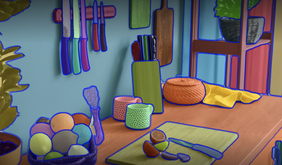
Figure 12: Meta’s Segment Anything semantic segmentation model
- 6D Pose Estimation enables precise robotic manipulation by providing the exact position ($x$, $y$, $z$) and orientation (roll, pitch, yaw) of objects in a scene. Modern approaches include: direct regression methods like PoseNet to keypoint-based approaches using PnP, while neural rendering techniques have emerged to handle challenging cases like symmetric and texture-less objects. Recent innovations in self-supervised learning and category-level pose estimation enable generalisation to novel objects29, while uncertainty estimation in pose predictions has become increasingly important for robust manipulation planning. Multi-view fusion techniques improve accuracy in complex scenarios, directly translating to more reliable and precise robotic manipulation capabilities in unstructured environments.
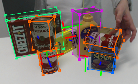
Figure 13: Deep Object Pose Estimation for Semantic Robotic Grasping of Household Objects NVIDIA
State Estimation
State estimation acts as a bridge between perception and control in robotics, enabling systems to maintain an accurate understanding of both their internal configuration and relationship to the environment. While classical approaches relied primarily on filtering techniques, modern methods increasingly combine traditional probabilistic frameworks with learned components to handle complex, high-dimensional state spaces and uncertainty quantification. This integration has proven particularly powerful for handling the non-linear dynamics and measurement noise inherent in robotic systems.
Sensor fusion in robotics integrates data from multiple sensors, including joint encoders, inertial measurement units (IMUs), and force-torque sensors, to accurately determine a robot’s internal configuration. Traditional approaches relied on simple Kalman filtering, modern robotics demands more sophisticated techniques to handle inherently non-linear system dynamics. Extended Kalman Filters (EKF) and Unscented Kalman Filters30 (UKF) address this challenge by performing recursive state estimation through linearization around current estimates. For applications requiring more robust handling of multi-modal distributions, particle filters offer an alternative solution, though at higher computational cost. Accurate sensor fusion is particularly critical for complex rigid robots, where precise joint state estimation directly impacts both control performance and operational safety.
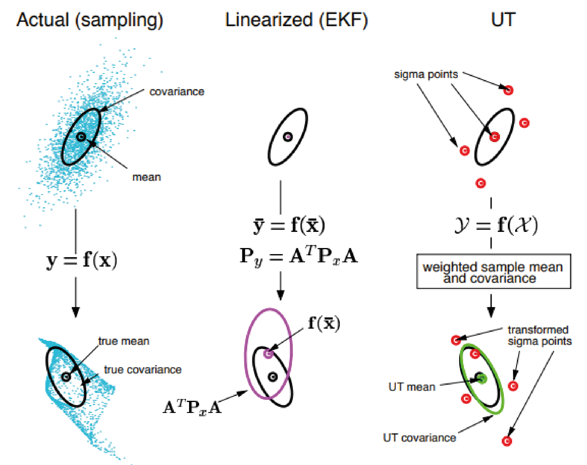
Figure 14: Comparison of Gaussian Transformations, from left to right. Actual Sampling captures the true mean and covariance, EKF approximates them with linearization, while the Unscented Transform (UT) uses sigma points for a more accurate nonlinear transformation.
Visual Inertial Odometry (VIO) enables mobile robots to estimate their motion by fusing visual and inertial data without relying on external reference points. Modern approaches like VINS-Fusion and ORB-SLAM3 achieve robust performance by tightly coupling feature-based visual tracking with inertial measurements. Deep learning has enhanced traditional VIO pipelines through learned feature detection, outlier rejection, and uncertainty estimation. End-to-end learned systems like DeepVIO31 demonstrate the potential of pure learning-based approaches, hybrid architectures have emerged as particularly effective, combining the reliability of geometric methods with the adaptability of learned components. These integrated systems are relatively mature and operate reliably in real-time while handling challenging real-world conditions including rapid movements32, variable lighting32, and dynamic obstacles33.
Figure 15: VINS-Fusion, visual-inertial state estimation for autonomous applications.
Factor graph optimisation provides a framework for sensor fusion and long-term state estimation in robotics. This approach represents both measurements and state variables as nodes in a graph structure, enabling efficient optimization over historical states to maintain consistency and incorporate loop closure constraints. Modern implementations like GTSAM and g2o have made these techniques practical for large-scale problems, while recent research has extended the framework to incorporate learned measurement factors. The field continues to advance through developments in robust optimisation34 for outlier handling, computationally efficient marginalisation schemes, and adaptive uncertainty estimation35. These theoretical advances have demonstrated practical impact in several robotic applications, including Simultaneous Localization And Mapping36 (SLAM) and object tracking.
Figure 16: GTSAM Structure from Motion
Citation
Quessy, Alexander. (2025). Robotic Learning for Curious People. aos55.github.io/deltaq. https://aos55.github.io/deltaq/posts/an-overview-of-robotic-learning/.
@article{quessy2025roboticlearning,
  title   = "Robotic Learning for Curious People",
  author  = "Quessy, Alexander",
  journal = "aos55.github.io/deltaq",
  year    = "2025",
  month   = "Feb",
  url     = "https://aos55.github.io/deltaq/posts/an-overview-of-robotic-learning/"
}
References
P. F. Hokayem and M. W. Spong, Bilateral Teleoperation: An Historical Survey. Cambridge, UK: Cambridge University Press, 2006. ↩︎
D. J. Reinkensmeyer and J. L. Patton, “Can Robots Help the Learning of Skilled Actions?,” Progress in Brain Research, 2009. ↩︎
K. Grauman, A. Westbury, E. Byrne, et al., “Ego4D: Around the World in 3,000 Hours of Egocentric Video,” IEEE Conference on Computer Vision and Pattern Recognition (CVPR), 2022. ↩︎
D. Damen, H. Doughty, G. M. Farinella, S. Fidler, A. Furnari, E. Kazakos, M. Moltisanti, J. Munro, T. Perrett, W. Price, and M. Wray, “EPIC-KITCHENS-100: Dataset and Challenges for Egocentric Perception,” IEEE Transactions on Pattern Analysis and Machine Intelligence, 2021. ↩︎
D. A. Pomerleau, “ALVINN: An Autonomous Land Vehicle in a Neural Network,” in Advances in Neural Information Processing Systems (NeurIPS), vol. 1, 1989. ↩︎
J. Ho and S. Ermon, “Generative Adversarial Imitation Learning,” in Advances in Neural Information Processing Systems (NeurIPS), vol. 29, 2016. ↩︎
S. Ross, G. Gordon, and D. Bagnell, “A Reduction of Imitation Learning and Structured Prediction to No-Regret Online Learning,” in Proceedings of the 14th International Conference on Artificial Intelligence and Statistics (AISTATS), 2011. ↩︎
D. Menda, M. Elfar, M. Cubuktepe, M. J. Kochenderfer, and M. Pavone, “ThriftyDAgger: Budget-Aware Novelty and Risk Gating for Interactive Imitation Learning,” in IEEE/RSJ International Conference on Intelligent Robots and Systems (IROS), 2020. ↩︎
J. Zhang and K. Cho, “Query-Efficient Imitation Learning for End-to-End Autonomous Driving,” in Advancement of Artificial Intelligence (AAAI), 2017. ↩︎
S. Ross and D. Bagnell, “Reinforcement and Imitation Learning via Interactive No-Regret Learning,” arXiv preprint arXiv:1406.5979, 2014. ↩︎
V. Mnih, K. Kavukcuoglu, D. Silver, A. A. Rusu, J. Veness, M. G. Bellemare, A. Graves, M. Riedmiller, A. K. Fidjeland, G. Ostrovski, et al., “Human-level control through deep reinforcement learning,” in Nature, vol. 518, no. 7540, pp. 529–533, 2015. ↩︎
J. Schulman, P. Moritz, S. Levine, M. Jordan, and P. Abbeel, “High-Dimensional Continuous Control Using Generalized Advantage Estimation,” in International Conference on Learning Representations (ICLR), 2016. ↩︎
J. Schulman, S. Levine, P. Abbeel, M. Jordan, and P. Moritz, “Trust Region Policy Optimization,” in International Conference on Machine Learning (ICML), 2015. ↩︎
J. Schulman, F. Wolski, P. Dhariwal, A. Radford, and O. Klimov, “Proximal Policy Optimization Algorithms,” arXiv preprint arXiv:1707.06347, 2017. ↩︎
T. Haarnoja, A. Zhou, P. Abbeel, and S. Levine, “Soft Actor-Critic: Off-Policy Maximum Entropy Deep Reinforcement Learning with a Stochastic Actor,” in International Conference on Machine Learning (ICML), 2018. ↩︎
H. van Hasselt, “Double Q-learning,” in Advances in Neural Information Processing Systems (NeurIPS), 2010. ↩︎
D. P. Kingma and M. Welling, “Auto-Encoding Variational Bayes,” in International Conference on Learning Representations (ICLR), 2014. ↩︎
L. M. Smith, I. Kostrikov, and S. Levine, “Demonstrating A Walk in the Park: Learning to Walk in 20 Minutes With Model-Free Reinforcement Learning,” in Proceedings of Robotics: Science and Systems (RSS), 2023. ↩︎
G. Williams, A. Aldrich, and E. Theodorou, “Model predictive path integral control: Information theoretic model predictive control,” in IEEE International Conference on Robotics and Automation (ICRA), 2017. ↩︎
K. Chua, R. Calandra, R. McAllister, and S. Levine, “Deep Reinforcement Learning in a Handful of Trials using Probabilistic Dynamics Models,” in Advances in Neural Information Processing Systems (NeurIPS), 2018. ↩︎
Sutton, R. S. “Dyna, an Integrated Architecture for Learning, Planning, and Reacting.” 1991. ↩︎
M. Janner, J. Fu, M. Zhang, and S. Levine, “When to Trust Your Model: Model-Based Policy Optimization,” in Advances in Neural Information Processing Systems (NeurIPS), 2019. ↩︎
N. Carion, F. Massa, G. Synnaeve, N. Usunier, A. Kirillov, and S. Zagoruyko, “End-to-End Object Detection with Transformers,” arXiv preprint arXiv:2005.12872, 2020. ↩︎
L. Qiao, Y. Zhao, Z. Li, X. Qiu, J. Wu, and C. Zhang, “DeFRCN: Decoupled Faster R-CNN for Few-Shot Object Detection,” arXiv preprint arXiv:2108.09017, 2021. ↩︎
L.-C. Chen, Y. Zhu, G. Papandreou, F. Schroff, and H. Adam, “Encoder-Decoder with Atrous Separable Convolution for Semantic Image Segmentation,” in European Conference on Computer Vision (ECCV), 2018. ↩︎
Z. Zhou, M. M. Rahman Siddiquee, N. Tajbakhsh, and J. Liang, “UNet++: A Nested U-Net Architecture for Medical Image Segmentation,” in Deep Learning in Medical Image Analysis and Multimodal Learning for Clinical Decision Support (DLMIA), 2018. ↩︎
R. Poudel, S. Liwicki, and R. Cipolla, “Fast-SCNN: Fast Semantic Segmentation Network,” in 2019 IEEE International Conference on Computer Vision (ICCV) Workshops, 2019, ↩︎
A. Kirillov, E. Mintun, N. Ravi, H. Mao, C. Rolland, L. Gustafson, T. Xiao, S. Whitehead, A. C. Berg, W.-Y. Chen, and P. Dollár, “Segment Anything,” arXiv preprint arXiv:2304.02643, 2023. ↩︎
B. Wen, W. Yang, J. Kautz, and S. Birchfield, “FoundationPose: Unified 6D Pose Estimation and Tracking of Novel Objects,” in Proceedings of the IEEE/CVF Conference on Computer Vision and Pattern Recognition (CVPR), 2024. ↩︎
E. A. Wan and R. van der Merwe, “The Unscented Kalman Filter for Nonlinear Estimation,” in Proceedings of the IEEE 2000 Adaptive Systems for Signal Processing, Communications, and Control Symposium (AS-SPCC), Lake Louise, Alberta, Canada, 2000. ↩︎
L. Han, Y. Lin, G. Du, and S. Lian, “DeepVIO: Self-supervised Deep Learning of Monocular Visual Inertial Odometry using 3D Geometric Constraints,” in 2019 IEEE/RSJ International Conference on Intelligent Robots and Systems (IROS), Macau, China, 2019. ↩︎
T. Qin, P. Li, and S. Shen, “VINS-Mono: A robust and versatile monocular visual-inertial state estimator,” IEEE Transactions on Robotics, 2018. ↩︎ ↩︎
B. Bescos, J. M. Fácil, J. Civera, and J. Neira, “DynaSLAM: Tracking, Mapping and Inpainting in Dynamic Scenes,” IEEE Robotics and Automation Letters, 2018. ↩︎
P. Agarwal, G. D. Tipaldi, L. Spinello, C. Stachniss, and W. Burgard, “Robust Map Optimization Using Dynamic Covariance Scaling,” in Proceedings of the IEEE International Conference on Robotics and Automation (ICRA), 2013. ↩︎
T. Naseer, M. Ruhnke, C. Stachniss, L. Spinello, and W. Burgard, “Robust Visual SLAM Across Seasons,” in Proceedings of the IEEE/RSJ International Conference on Intelligent Robots and Systems (IROS), 2015. ↩︎
C. Cadena, L. Carlone, H. Carrillo, Y. Latif, D. Scaramuzza, J. Neira, I. Reid, and J. J. Leonard, “Past, Present, and Future of Simultaneous Localization and Mapping: Toward the Robust-Perception Age,” IEEE Transactions on Robotics, 2016. ↩︎