Imagine teaching a robot to pick up a coffee cup in a simulation or video game. In this perfect virtual world, the cup’s weight is precisely known, the lighting is consistent, and the robot’s sensors provide exact measurements. Now try the same task in the real world. The cup might be heavier than expected, it’s surface more slippery, the lighting creating unexpected shadows, and the robot’s sensors noisy. This disconnect between simulation and reality, known as the reality gap, is a fundamental challenge in robotic learning.
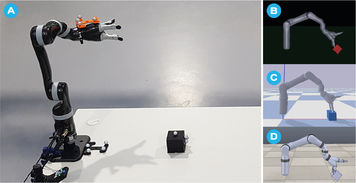
Figure 1: Example of real-world and simulated environments for training a Kinova Arm.
The appeal of simulation is clear: we can attempt thousands of trials in parallel, experiment without risk of spilling coffee or breaking cups, easily reset the simulation to any starting state, and generate unlimited training data. In-fact it is probably safe to say robotic learning as we know it today would be impossible without simulators. But simulations are approximations and can’t perfectly capture the physics of gripping a cup, the variations in cup shapes and materials, or the complexities of real-world sensor noise. This creates a problem:
How do we ensure that skills learned in simulation transfer effectively to the real world?
Researchers have developed three main approaches to address this challenge:
- Improving Simulation Fidelity: Making simulations more realistic, so there is less of a mismatch between the policy learned in simulation and in the real-world.
- Learning Robust Policies: Developing algorithms that are inherently adaptable by accounting for sim-to-real differences during training.
- Online Adaptation: Enabling policies to efficiently adjust to real-world conditions by online fine-tuning.
Making Simulations more Realistic
One approach to bridging the reality gap is to design simulators that better match the real world. The intuition behind why this works is straightforward:
The smaller the difference between simulation and reality, the smaller the reality gap that must be bridged.
If a robot learns to grasp in a highly accurate simulation that captures subtle physical properties like friction coefficients, contact dynamics, and fluid interactions, those skills are more likely to transfer successfully to the real world. However, creating perfect simulations is impossible, there will always be some mismatch with reality. As George Box said, famously:
All models are wrong; some are useful. - George Box
But which aspect of reality matters most? Most engineers would be familiar with this approach as defining a problems assumptions or boundary conditions before designing a model. For example in grasping tasks, accurate contact dynamics and friction modelling might be essential, whilst precise visual rendering of shadows is less important. In contrast, for vision-based navigation, accurate lighting models could be critical while precise physics are less important.
System Identification
System Identification aims to calibrate the parameters within a simulation to match real-world behaviour. This process aims to find the optimal parameters $\mathbf{\xi}^{*}$ that minimise the difference between simulated and real trajectories:
$$ \mathbf{\xi}^{*} = \arg \min_{\mathbf{\xi}} \sum_{t=1}^{T} || s_{t}^{\text{real}} - s_{t}^{sim}(\mathbf{\xi}) || $$where $s_{t}^{\text{real}}$ are real-world observations and $s_{t}^{\text{sim}}(\mathbf{\xi})$ are simulated states using parameters $\mathbf{\xi}$.
This process generally involves:
- Collecting real robot trajectories and sensor measurements.
- Selecting simulator parameters (mass, friction coefficients, motor gains, etc) to minimise the difference between the simulated and real-world behaviour.
- Iteratively refining these parameters as more data becomes available.
While system identification is a powerful approach, it poses unique challenges for learned robotics. The parameters we’re trying to identify are deeply intertwined with the learning process itself. As a policy learns and explores new regions of the state space, it encounters different dynamic regimes that may require different parameter values for accurate simulation. This creates a chicken-and-egg problem: we need accurate parameters to learn good policies, but we need policies to explore and gather data for parameter identification. Furthermore, learned policies often exploit subtle dynamics that aren’t captured by standard physics models, making it difficult to identify parameters that consistently work across the full range of learned behaviours. This is particularly challenging for contact-rich tasks like manipulation, where small parameter errors can lead to drastically different outcomes in both the learning process and final policy behaviour.
Larger vehicles, such as planes1, trains and automobiles, that may have high order but generally parameterisable and smooth dynamics system id is often used. For more complex robots the non-linear dynamics introduced by the real-world often pose a challenge and can make system id impractical.
Learned Simulation
Rather than manually tuning parameters, learned simulation uses real-world data to improve simulator accuracy directly. The main idea is that while physics-based simulators capture fundamental dynamics well, they often miss subtle effects that are difficult to model analytically. Learning can be used to bridge this gap.
Residual Dynamics
One approach is to learn a residual dynamics model. These models work by combining a base physics model with a learned component that predicts the difference between the simulated and real-world behaviour. Formally, given a base simulator $f_{\text{sim}}(s_{t}, a_{t})$ and true dynamics $f_{\text{real}}(s_{t}, a_{t})$, we learn a residual model $f_{\text{res}}(s_{t}, a_{t})$ such that:
$$ f_{\text{real}} \approx f_{\text{sim}}(s_{t}, a_{t}) + f_{\text{res}}(s_{t}, a_{t}). $$This approach2 can be very effective3 because it leverages the prior knowledge of the physics simulator, which is often a far cheaper and easier problem to solve than learning a complete simulator from scratch. For example, in our coffee cup grasping task, the base simulator could handle rigid body dynamics, while the residual learns to correct for joint backlash, motor delays, and complex friction effects.
Differentiable Physics
In most of the robotic learning approaches discussed so far we assumed the algorithm learns through trial and error. In our coffee cup example this might involve the robot sometimes gripping too hard and crushing the cup, and sometimes gripping too softly and dropping it. After hundreds or thousands of attempts, it should eventually learn a useful grasp strategy.
Imagine instead having a mathematical model that can instantly tell the robot: “If you move your finger $2mm$ to the left and reduce gripping force by $4.2\text{N}$ the cup will be stable in your grasp without being crushed”. This is what differentiable physics simulators offer for robotic learning.
A differentiable physics simulator creates a mathematical model where every physical interaction, can be calculated and, critically, differentiated. This means the robot can compute exactly how small changes in its actions will affect the outcome of grasping the cup.
Unlike traditional physics engines with non-differentiable components (like discrete collision detection), differentiable simulators express physical laws as continuously differentiable operations. This mathematical property allows for gradient-based optimisation through the entire physical process, effectively letting the robot “see into the future” to optimise its actions.
Mathematically, the physics simulator implements a transition function $f$:
$$ s_{t+1} = f(s_{t}, a_{t}, \xi). $$The simulator then provides the Jacobian matrices:
$$ \biggl[ \frac{\partial s_{t+1}}{\partial s_{t}}, \frac{\partial s_{t+1}}{\partial a_{t}}, \frac{\partial s_{t+1}}{\partial \xi_{t}} \biggr]. $$These matrices tell us how small changes in the current state, action, or parameters $\theta$ affect the next state. When optimising over time, BackPropagation Through Time (BPTT) allows gradients to be rolled out for the entire sequence. Enabling the robot to understand how its initial actions influence the final outcome. This is particularly valuable for contact-rich tasks where traditional simulators struggle with discontinuities in the dynamics.
To actually learn a policy gradient-based optimisation algorithms are often used including:
- Policy Optimisation 4, can be used by back-propagating through the simulator: $$ \nabla_{\theta}J(\xi) = \mathbb{E}_{\xi \sim \Xi} \bigl[ \nabla_{\theta} f(s, a; \xi) \bigr]. $$ The gradient of the objective with respect to the policy parameters can be directly computed, rather than relying on purely numerical approximations.
- MPC w/ Differentiable Shooting5, unlike traditional MPC, which relies on solving an optimisation problem at each time-step, this approach differentiates through the entire trajectory 6 : $$ \min_{a_{0:T-1}} \sum_{t=0}^{T-1} c(s_{t}, a_{t}) + c_{T}(s_{T}). $$
- Trajectory Optimisation, gradient based optimisation techniques like Differential Dynamic Programming (DDP) or iterative Linear Quadratic Regularisation (iLQR) become more powerful with differentiable physics as they can compute the exact derivatives of the dynamics rather than using numerical finite difference methods.
Figure 2: DiffTaichi differentiable programming for physical simulation.
Recent frameworks like Brax, Nimble, and DiffTaichi implement efficient differentiable physics that integrate seamlessly with deep learning workflows. For robotics applications, differentiable simulation enables more efficient policy learning, automated system identification, and even physics-based perception, where sensor models can be optimised alongside control policies.
Figure 3: Brax differentiable physics simulator for robotics written in JAX.
Domain Randomisation
Instead of trying to make the simulation perfect, Domain Randomisation7 (DR) encourages imperfection by training with varying simulation parameters. The main idea is that by exposing the policy to a wide range of simulator variations during training, it will learn to focus on task-relevant features while being robust to variations that don’t matter.
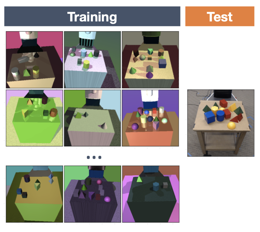
Figure 4: Domain Randomisation was orginially designed with the objective of training an object detector.
Mathematically, we can express this as training a policy $\pi$ to maximise expected performance across a distribution of environments:
$$ \pi^{*} = \arg \max_{\pi} \mathbb{E}_{\xi \sim p(\xi)} [J(\pi, \xi)] $$where $\xi$ represents simulator parameters and $J(\pi, \xi)$ is the performance of a policy $\pi$ in the environment.
The main idea is that if we randomise enough aspects of the simulation, the real world becomes one possible outcome among many in the distribution. DR is particularly effective because it naturally produces policies robust to real-world variations, eliminates the need for precise physics modelling and requires no real-world training data.
For the coffee cup example, rather than trying to perfectly model the cup DR might vary:
- Physical Properties: mass, friction.
- Visual Properties: cup colours, textures, lighting conditions.
- Sensor Properties: camera noise, force sensor bias.
- Robot Properties: joint backlash, motor delays.
To practically use DR the parameter ranges and distribution types need to be selected carefully. Too broad and the learning process can become inefficient, too narrow and the policy won’t be general enough to adapt to the real-world.
This challenge has led to advanced techniques like adaptive randomisation (automatically tuning ranges based on performance) and structured randomisation (using domain knowledge to guide parameter variations). The core principle remains:
By training across many simulated variations, we can learn policies that transfer to the real world without requiring perfect simulation.
Learning Strategies for Transfer
While improving simulation fidelity helps bridge the reality gap, we can also design learning algorithms that are inherently robust to the sim-to-real transition. Rather than assuming perfect simulation, these approaches focus on learning representations and policies that transfer effectively despite simulation imperfections.
Domain Adaption
Domain adaption8 aims to bridge the sim-to-real gap by teaching robots to recognise and adapt to discrepencies between simulated and real environments. This approach focuses on learning transformations that align the data distributions from both domains. The core idea is simple yet powerful:
Train the robot to focus on features that work consistently across both simulation and reality, while ignoring features that differ between them.
For instance, the robot should learn that the general shape of a cup is important for grasping, while slight differences in texture or lighting are irrelevant.
Mathematically, domain adaptation works by training neural networks to extract features that minimise the distributional difference between simulation and reality. Formally, given a feature extractor $f_{\theta}$, we aim to learn features where the distributions match:
$$ \min_{\theta} D \bigl( f_{\theta}(x_{sim}) || f_{\theta}(x_{real}) \bigr) $$where $D$ measures the distributional distance, such as KL-divergence.
This is often implemented using adversarial training, similar to Generative Adversarial Nets9 (GANs). A discriminator network tries to determine whether features came from simulation or reality, while the feature extractor aims to make this distinction impossible:
$$ \min_{\theta} \max_{D} \mathbb{E}_{x_{\text{sim}}} \Bigl[ \log D \bigl( f_{\theta}(x_{\text{sim}}) \bigr) \Bigr] + \mathbb{E}_{x_{\text{real}}} \Bigl[ 1 - \log D \bigl(f_{\theta} ( x_{\text{real}}) \bigr) \Bigr] . $$For adversarial domain randomisation, we go a step further by learning a distribution of simulator parameters $p(\xi)$ that, ideally, produces data indistinguishable from reality:
$$ \min_{p(\xi)} \max_{D} \mathbb{E}_{\xi \sim p(\xi)} \Bigl[ \log D \bigl( x_{\text{sim}}(\xi) \bigr) \Bigr] + \mathbb{E}_{x_{\text{real}}} \Bigl[ 1 - \log D \bigl(f_{\theta} ( x_{\text{real}}) \bigr) \Bigr] . $$In practice, this means our coffee-cup-grasping robot learns representations that work equally well in simulation and reality. When transferred to the real world, the robot focuses on the aspects of cup-grasping that remain consistent, making the sim-to-real transition much smoother.
These methods typically require some real-world data, and can be used in a sim-to-real-to-sim10 cycle. In this framework, policies trained in simulation are deployed in the real-world, and the collected data improves the simulation for subsequent iterations. This cyclical approach creates increasingly robust representations with each iteration. Domain adaptation is particularly powerful when combined with other sim-to-real techniques, as it directly addresses the distributional gap while remaining compatible with methods focused on policy robustness or online adaptation.
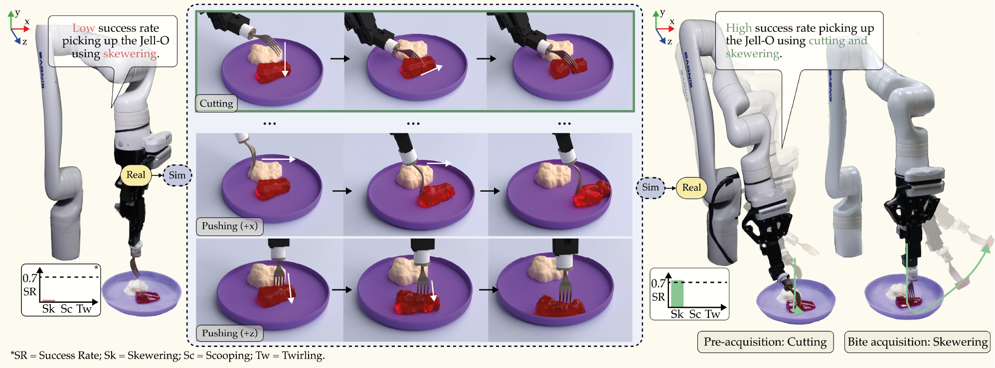
Figure 5: REPeat uses a Real2Sim2Real approach to improve robot-assisted feeding.
Meta Learning
Meta-learning offers an alternative approach to the sim-to-real challenge. Rather than focusing on improving simulator fidelity or training robust policies in simulation, meta-learning takes a fundamentally different approach:
Train the robot to quickly adapt to new situations with minimal data.
Think of it as learning adaptability.
For our coffee cup example, instead of training a robot to master grasping a specific cup in simulation (which may not transfer well to reality), meta-learning trains the robot to understand general grasping principles that enable rapid adaptation when encountering real cups with varying properties, textures, and weights using just a few real-world interactions. The emphasis shifts from perfecting the simulation to developing algorithms that can bridge the reality gap through efficient learning.
Mathematically meta-learning can be expressed as a two-level optimisation problem:
$$ \min_{\theta} \mathbb{E}_{\mathcal{T} \sim p(\mathcal{T})} [\mathcal{L}_{\mathcal{T}}(A(\theta, \mathcal{T}))] $$where $\theta$ is a parameterised policy, $p(\mathcal{T})$ is a distribution over tasks or environments, $A(\theta, \mathcal{T})$ is an adaption process that adjusts $\theta$ for a specific task, and $\mathcal{L}_{\mathcal{T}}$ measures the performance on a task $\mathcal{T}$.
This formulation summarises the main idea behind meta-learning, we optimise not for direct task performance but on how well the robot can adapt when facing new situations. For sim-to-real, this can be described as the following process:
$$ \begin{align*} & \textbf{Meta-Learning for Sim2Real Transfer} \\ & \\ & \textbf{Initialize:} \\ & \quad \text{Meta-parameters: } \theta \\ & \quad \text{Adaptation procedure: } A(\theta, \mathcal{D}) \\ & \quad \text{Task distribution: } p(\mathcal{T}) \text{ over simulation parameters} \ \xi \\ & \\ & \textbf{Simulated Meta-Training:} \\ & \textbf{for } \text{iteration} = 1,\dots,N \textbf{ do:} \\ & \quad \text{Sample batch of tasks } \{\mathcal{T}_1,\dots,\mathcal{T}_k\} \sim p(\mathcal{T}) \\ & \quad \textbf{for each } \mathcal{T}_i \textbf{ do:} \\ & \quad\quad \text{Collect simulation trajectories } \mathcal{D}_i \\ & \quad\quad \text{Split into } \mathcal{D}^{\text{train}}_i, \mathcal{D}^{\text{test}}_i \\ & \quad\quad \text{Adapt parameters: } \theta_i = A(\theta, \mathcal{D}^{\text{train}}_i) \\ & \quad\quad \text{Evaluate adapted parameters: } \mathcal{L}_{\mathcal{T}_i}(\theta_i, \mathcal{D}^{\text{test}}_i) \\ & \quad \text{Update } \theta \text{ to minimize } \mathbb{E}_{\mathcal{T}_i}[\mathcal{L}_{\mathcal{T}_i}(\theta_i, \mathcal{D}^{\text{test}}_i)] \\ & \textbf{end for} \\ & \\ & \textbf{Real-World Deployment:} \\ & \quad \text{Collect small real-world dataset } \mathcal{D}_\text{real} \\ & \quad \text{Adapt to real world: } \theta_\text{real} = A(\theta, \mathcal{D}_\text{real}) \\ & \quad \text{Deploy adapted policy } \pi_{\theta_\text{real}} \text{ in real environment} \\ \end{align*} $$In robotics, optimisation based meta-learning approaches have gained the most attention, often based on the Model Agnostic Meta Learning11 (MAML) algorithm. Unlike model-based methods that attempt to learn explicit task dynamics or metric-based approaches that rely on learned distance measures between tasks, MAML directly optimises for adaptability through a gradient-based formulation:
$$ \min_{\theta} \mathbb{E}_{\mathcal{T} \sim p(\mathcal{T})} [\mathcal{L}_{\mathcal{T}}(\theta - \alpha \nabla_{\theta} \mathcal{L}_{\mathcal{T}}(\theta))]. $$For robotic applications, MAML’s gradient-based adaptation mechanism integrates naturally with deep learning architectures and standard reinforcement learning objectives. While model-based approaches must learn accurate dynamics models, which can be challenging for complex robotic systems, and metric-based approaches require carefully designed embedding spaces, MAML works directly in parameter space. This allows it to capture sophisticated adaptation strategies without additional architectural constraints.
Figure 6: ES-MAML uses Evolutionary Strategies (ES) to learn an adaptive control policy for a noisy task.
Also, the computation of MAML’s adaptation gradients $\nabla_{\theta}\mathcal{L}_{\mathcal{T}}(\theta)$ can leverage standard automatic differentiation tools, making it easy to implement despite its mathematical sophistication. Often a first-order approximation (FOMAML) is used to improve computational efficiency by ignoring second-order terms in the meta-gradient computation, while still maintaining much of the method’s adaptation capabilities.
While MAML provides efficient adaptation through gradient-based updates, it doesn’t explicitly model uncertainty in the task parameters, a critical consideration for sim-to-real transfer, where real-world dynamics are initially unknown. Probabilistic meta-learning12 approaches address this limitation by modelling a distribution over possible task parameters:
$$ p(\mathcal{T}|\mathcal{D}) = \int p(\mathcal{T}|\theta) p(\theta|\mathcal{D}) d \theta . $$This allows the robot to maintain and update beliefs about real-world dynamics as it collects data. Probabilistic Embeddings for Actor-Critic RL13 (PEARL) builds on this insight by combining meta-learning with probabilistic inference. Instead of MAML’s direct parameter adaptation, PEARL learns a latent space of task variables that capture task uncertainty:
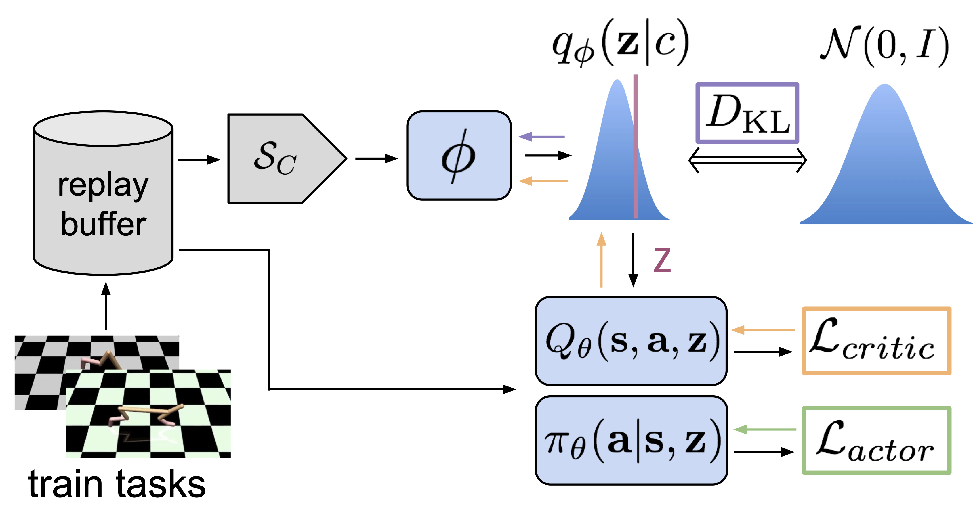
Figure 7: PEARL’s meta-training procedure.
Here, the policy $\pi_{\theta}$ conditions its actions not just on the current state $s$, but also on a latent task variable $z$ inferred from task-specific data $\mathcal{D}_{\mathcal{T}}$. This structure provides several advantages for sim-to-real transfer:
- The learned latent space can capture structured uncertainty about task parameters, allowing for more efficient exploration than MAML’s gradient-based adaptation.
- By learning a probabilistic encoder $q_{\phi}$, usually via a Variational Auto-Encoder14 (VAE), PEARL can rapidly infer task-relevant parameters from small amounts of real-world data without requiring gradient updates to the policy parameters. This uncertainty-aware approach enables robots to systematically explore and adapt to real-world conditions while maintaining uncertainty estimates about task dynamics.
Modular Policy Architectures
Rather than treating sim-to-real transfer as a monolithic problem, modular architectures break policies into components that can be transferred or adapted independently. This decomposition allows us to leverage the fact that some aspects of a task may transfer more readily than others. End-to-end systems are also notoriously hard to debug and breaking the problem down into smaller sub-problems can help to identify exactly what part of the system is misbehaving. Robotic tasks often naturally decompose into three main components:
- Perception, understanding the environment through sensors.
- Planning, deciding what actions to take.
- Control, precisely executing these actions.
Perception modules face domain gaps between clean simulation data and noisy reality. For example, when detecting objects with RGB cameras, simulated images often lack real-world artefacts like motion blur, lens distortion, and varying exposure levels. Some techniques to address this could include:
- Using synthetic data augmentation with Physically-Based Rendering (PBR) to match real camera characteristics.
- Implementing CycleGAN-based domain adaptation15 to align synthetic and real image distributions.
- Applying targeted domain randomisation to critical visual features like lighting and camera parameters.
Planning modules need to handle state uncertainty when moving from simulation to reality. Some methods to solve this include:
- Using belief space planning16 that explicitly considers state uncertainty distributions.
- Implementing hierarchical17 planning with closed-loop feedback at multiple timescales.
- Incorporating learned error models18 that predict the magnitude and distribution of real-world deviations from planned trajectories.
Control modules must bridge the reality gap in physical interactions. Some methods to solve this include:
- Structured Domain Randomisation19 (SDR), systematically varying physical parameters based on the specific hardware used. This method can also be used for perception problems.
- Learning-Based Model Predictive Control20 (LBMPC), combining traditional MPC with learned vehicle dynamics.
- Meta-Learning for Rapid Control Adaptation21.
These modular approaches work best when combined with other transfer strategies, like using meta-learning to adapt specific modules or applying domain adaptation selectively. This flexibility in mixing approaches makes modularity a particularly effective tool for bridging the reality gap and can better scale when building robotic systems with a larger team or group where departments need to focus on separate components and end-to-end learning would be infeasible.
Online Adaption and Deployment
While training in simulation and transfer learning provide essential components for robotic learning, the reality of real-world deployment often presents challenges that cannot be fully anticipated. Environmental variations, hardware differences between robots, and changing task requirements all necessitate real-world adaptation. Online adaptation enables robots to continuously refine their policies during actual deployment, adjusting to real-world conditions that may drift over time or differ from training assumptions.
The key challenge in online adaptation is balancing the need for exploration and improvement against maintaining reliable performance and safety. Unlike simulation, where exploration carries no physical risk, real-world adaptation must be conducted carefully to avoid expensive or dangerous failures. This creates a complex trade-off:
Adapt too conservatively and the robot may never achieve optimal performance, adapt too aggressively and you risks unsafe behaviour.
Modern approaches to online adaptation address this challenge through several complementary strategies. Few-shot adaptation enables rapid policy updates using minimal real-world data. Lifelong learning methods allow robots to accumulate experience while preventing degradation of existing capabilities. Progressive transfer techniques provide structured frameworks for safely transitioning from simulation to real-world operation. Importantly, these approaches must also consider practical deployment constraints like computational resources, hardware variations between robots, and the potential for knowledge sharing across robotic fleets.
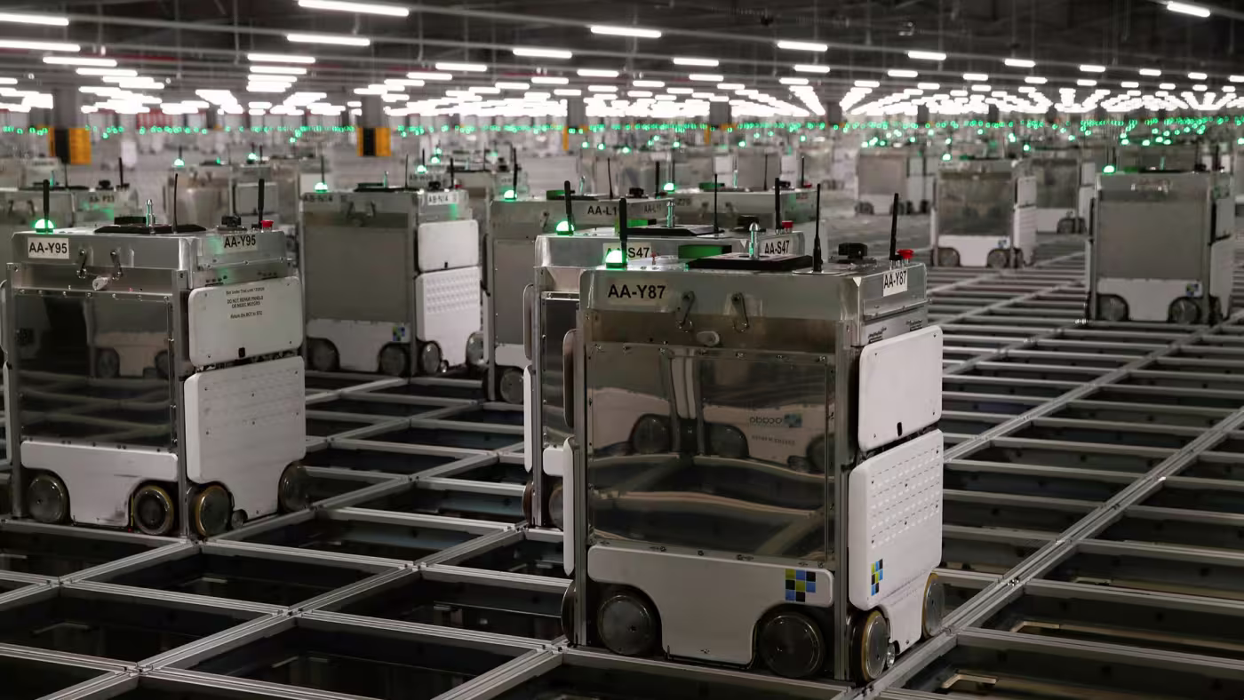
Figure 9: UK online food retailer Ocado’s robotic food packing robots.
Few-Shot Adaption
Online adaptation in robotics often requires making policy adjustments with small quantities of real-world data. Few-shot adaptation techniques address this challenge by enabling rapid policy updates using just a handful of real-world interactions, making them particularly valuable when collecting extensive real-world data is expensive or dangerous. While meta-learning approaches train policies to be inherently adaptable before deployment, few-shot adaptation22 focuses on efficient policy refinement during actual deployment.
One strategy, used by SafeAPT23, is to maintain an ensemble of policies trained in simulation, then adapt their combination based on real-world performance:
$$ \pi_{\text{adapted}}(a|s) = \sum_{i=1}^{N} w_{i}(s) \pi_{i}(a|s) $$where $w_{i}(s)$ is the context-dependent weights updated online using real-world data. This approach allows robots to leverage diverse behaviours, learned in simulation while quickly adapting their mixture to specific operating conditions. The weights can be rapidly updated using techniques like Bayesian inference or online optimisation, requiring only a few real-world samples.
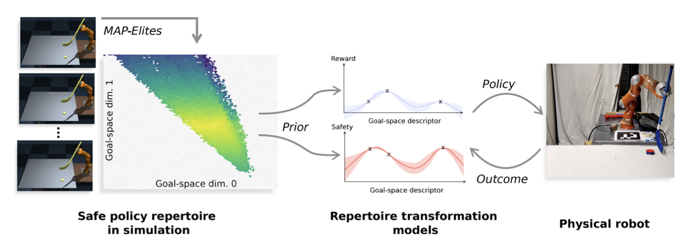
Figure 8: SafeAPT generates a diverse repertoire of safe policies in simulation, then selects and refines the most suitable policy for real-world goals using a learned safety model.
For multi-robot systems, few-shot adaptation24 can be enhanced through shared learning. When one robot successfully adapts to a new situation, its new experience can be validated and shared across the fleet:
$$ \mathcal{D}_{\text{shared}} = \{ (s, a, r, c)_{i} : V(s, a, c) > \tau \} $$where $V(s,a,c)$ is a validation function that evaluates the safety and performance of state-action pairs under context $c$, and $\tau$ is a safety threshold. This allows the fleet to collectively adapt to new situations while maintaining safety guarantees25.
Hardware variations between robots present an additional challenge for few-shot adaptation. One approach is to learn hardware-specific adaptation layers while maintaining a shared base policy:
$$ \pi_{\text{robot}}(a|s) = h_{\phi}(\pi_{\text{base}}(s), \xi) $$where $h_{\phi}$ is a hardware-specific adaptation layer and $\xi$ represents hardware parameters such as actuator limits, sensor characteristics, and physical dimensions. This architecture allows each robot to quickly adapt to its specific hardware characteristics26 while leveraging shared knowledge.
Any shared learning framework requires robust validation27 mechanisms. During few-shot learning, runtime monitoring systems can be used to continuously evaluate adapted behaviors against key performance indicators and safety constraints:
$$ \text{safe}(s, a) = \forall i \in \{ 1, \ldots , M \} : C_{i}(s, a) \leq 0 $$where $C_{i}$ represent safety constraints. When a robot discovers a promising adaptation, the validation function $V(s,a,c)$ determines whether this experience merits inclusion in the shared dataset $\mathcal{D}_{\text{shared}}$. If constraint violations occur during deployment, the system can revert to a known safe policy while collecting data for more robust adaptation. This closed-loop validation approach ensures that the collective learning process remains safe and reliable even as the robot fleet explores new adaptation strategies.
Real-world examples of fleet learning systems with these validation mechanisms remain scarce in public literature, as they’re typically proprietary technologies developed by companies like Waymo, Boston Dynamics, and Amazon Robotics. There is an increasing amount of open-source research for fleet adaptation systems, but these are often limited to small-scale experiments28.
Lifelong Learning
While few-shot adaptation handles immediate adjustments, lifelong learning focuses on continuous improvement during extended deployment. This presents a fundamental challenge:
How can robots accumulate new knowledge over months or years of operation without forgetting their existing capabilities?
A key challenge of this trade-off is catastrophic forgetting29. This is particularly important in robotics, where maintaining baseline performance while learning is essential for practical deployment. It is especially challenging in task-agnostic settings where task boundaries are unclear, and the robot must continuously learn without explicit transitions between distinct learning phases that you might have in classical ML setups.
Regularisation based methods offer one approach to mitigate catastrophic forgetting. Techniques like Elastic Weight Consolidation30 (EWC) identify and protect important parameters for previously learned tasks by adding constraint terms to the loss function:
$$ \mathcal{L}_{\text{EWC}}(\theta) = \mathcal{L}_{\text{current}}(\theta) + \sum_{i} \frac{\lambda}{2} F_{i}(\theta - \theta_{\text{A, i}}^{*})^{2} $$where $\mathcal{L}_{\text{current}}(\theta)$ represents the loss for the current task, $\lambda$ describes how important the old task is compared to the new one, and $F_{i}$ is the Fisher information representing parameter importance for task $i$ where $\theta_{A, i}$ is the optimal parameters for the previous tasks.
Replay based methods can also be used, such as Prioritized Experience Replay31 (PER), that maintains a buffer of past-experiences $\mathcal{B}$ with a priority weight $\alpha(s, a)$. $\delta(s, a)$ is the temporal difference error that quantifies how much the current policy’s predictions deviate from observed rewards and state transitions. The sampling probability is given by:
$$ P(i) = \frac{p_i^{\alpha}}{\sum_k p_k^{\alpha}} $$where $\alpha$ determines how much prioritization is used. To correct for sampling bias, importance sampling weights $w_i = (N \cdot P(i))^{-\beta}$ are applied to the loss gradients.
The learned architecture can also be adjusted to inherently resist forgetting. For example, Progressive Neural Networks32 (PNN) expand the architecture for each new task while preserving previous learned knowledge. PackNet33 partitions network parameters across tasks to prevent interference.
For all of these strategies the fundamental challenge remains balancing plasticity (the ability to learn new tasks) with stability (retaining performance on previous tasks). Systems that lean too far toward stability resist new learning, while those prioritizing plasticity risk catastrophic forgetting. Modern approaches often use a blend of these approaches, for example predictive uncertainty estimates34 can be used to decide how samples should be included in the model whilst learning online.
Complementary to addressing forgetting, efficient memory management is important in the real world. Real robots cannot store petabytes of raw-experience data, and blindly replay all past-experiences as this is simply too expensive and can limit exploration.
Lifelong learning is a complex and rapidly evolving field that deserves more detail than I can provide in this section. As companies scale robotic deployments across more locations with increasingly sophisticated behaviors, I expect we’ll discover much more about the specific engineering challenges involved.
Progressive Transfer
Progressive transfer provides a structured approach for transitioning policies from simulation to real-world operation. Rather than attempting an immediate switch, robots gradually reduce their reliance on simulation while building confidence in real-world performance. This approach is particularly important for safety-critical applications and fleet-wide deployments.
The core idea usually blends simulation and real-world policies based on deployment confidence:
$$ a_{\text{final}}(s,c) = (1-\beta(s,c))a_{\text{real}}(s) + \beta(s,c)a_{\text{sim}}(s) $$where $\beta(s, c) \in [ 0, 1 ]$ represents confidence in the real-world policy for state $s$ and context $c$. As deployment experience increases and safety metrics improve, $\beta$ decreases, shifting control from simulation-based to real-world policies. Context $c$ captures task complexity, environmental conditions, and safety requirements.
Summary
I hope this section has helped provide some useful insights into why sim2real is important for real-world robotics. This has proven to be the hardest part of this blog post to write, and I would like to expand in the future on the real-world deployment challenges of the sim2real problem. Just as we have learned that moving ML from the lab to scaled businesses has created its own host of ML problems, I’m sure we will continue to see similar challenges with moving robotic learning to scale.
Citation
Quessy, Alexander. (2025). Robotic Learning for Curious People. aos55.github.io/deltaq. https://aos55.github.io/deltaq/posts/an-overview-of-robotic-learning/.
@article{quessy2025roboticlearning,
  title   = "Robotic Learning for Curious People",
  author  = "Quessy, Alexander",
  journal = "aos55.github.io/deltaq",
  year    = "2025",
  month   = "June",
  url     = "https://aos55.github.io/deltaq/posts/an-overview-of-robotic-learning/"
}
References
K W Liff, Parameter Estimation for Flight Vehicles, Journal of Guidance, Control and Dynamics, 1989. ↩︎
N Sontakke, H Chae, S Lee, T Huang, D W. Hong, S Ha, Residual Physics Learning and System Identification for Sim-to-real Transfer of Policies on Buoyancy Assisted Legged Robots, arXiv:2303.09597, 2023. ↩︎
H Jemin, L Joonho, H Marco, Per-Contact Iteration Method for Solving Contact Dynamics, IEEE Robotics and Automation Letters, 2018. ↩︎
H.J. Terry Suh, Max Simchowitz, Kaiqing Zhang, Russ Tedrake, Do Differentiable Simulators Give Better Policy Gradients?, Proceedings of the 39th International Conference on Machine Learning, PMLR 162, 2022. ↩︎
A. Romero, E. Aljalbout, Y. Song, D. Scaramuzza, Actor-Critic Model Predictive Control: Differentiable Optimization Meets Reinforcement Learning, arXiv:2306.09852, 2024. ↩︎
A. Oshin, H. Almubarak, E.A. Theodorou, Differentiable Robust Model Predictive Control, Robotics: Science and Systems, Delft, Netherlands, 2024. ↩︎
J. Tobin, R. Fong, A. Ray, J. Schneider, W. Zaremba, P. Abbeel, Domain Randomization for Transferring Deep Neural Networks from Simulation to the Real World, arXiv:1703.06907, 2017. ↩︎
Y. Ganin, V. Lempitsky, Unsupervised Domain Adaptation by Backpropagation, Proceedings of the 32nd International Conference on Machine Learning (ICML), 2015. ↩︎
I.J. Goodfellow, J. Pouget-Abadie, M. Mirza, B. Xu, D. Warde-Farley, S. Ozair, A. Courville, Y. Bengio, Generative Adversarial Nets, Proceedings of the 27th International Conference on Neural Information Processing Systems (NIPS), 2014. ↩︎
S. James, P. Wohlhart, M. Kalakrishnan, D. Kalashnikov, A. Irpan, J. Ibarz, S. Levine, R. Hadsell, K. Bousmalis, Sim-to-Real via Sim-to-Sim: Data-efficient Robotic Grasping via Randomized-to-Canonical Adaptation Networks, Proceedings of the IEEE/CVF Conference on Computer Vision and Pattern Recognition (CVPR), 2019. ↩︎
C. Finn, P. Abbeel, and S. Levine, “Model-Agnostic Meta-Learning for Fast Adaptation of Deep Networks,” Proceedings of the 34th International Conference on Machine Learning, 2017. ↩︎
C. Finn, K. Xu, and S. Levine, “Probabilistic Model-Agnostic Meta-Learning,” Proceedings of the 31st Conference on Neural Information Processing Systems (NeurIPS 2017), 2017. ↩︎
K. Rakelly, A. Zhou, D. Quillen, C. Finn, and S. Levine, “Efficient Off-Policy Meta-Reinforcement Learning via Probabilistic Context Variables,” Proceedings of the 36th International Conference on Machine Learning (ICML), 2019. ↩︎
D. P. Kingma and M. Welling, “Auto-Encoding Variational Bayes,” Proceedings of the 2nd International Conference on Learning Representations (ICLR) 2014. ↩︎
K. Rao, C. Harris, A. Irpan, S. Levine, J. Ibarz, and M. Khansari, “RL-CycleGAN: Reinforcement Learning Aware Simulation-To-Real,” Conference on Computer Vision and Pattern Recognition (CVPR), 2020. ↩︎
S. Patil, G. Kahn, P. Abbeel, and 3 other authors, “Scaling up Gaussian Belief Space Planning Through Covariance-Free Trajectory Optimization and Automatic Differentiation,” Workshop on the Algorithmic Foundations of Robotics (WAFR 2014), 2014. ↩︎
T. D. Kulkarni, K. R. Narasimhan, A. Saeedi, and J. B. Tenenbaum, “Hierarchical Deep Reinforcement Learning: Integrating Temporal Abstraction and Intrinsic Motivation,” Proceedings of the 30th Conference on Neural Information Processing Systems (NeurIPS), Dec. 2016. ↩︎
A. Sharma, J. Harrison, M. Tsao, and M. Pavone, “Robust and Adaptive Planning under Model Uncertainty,” Proceedings of the Twenty-Ninth International Conference on Automated Planning and Scheduling (ICAPS 2019), 2019. ↩︎
A. Prakash, S. Boochoon, M. Brophy, D. Acuna, E. Cameracci, G. State, O. Shapira, and S. Birchfield, “Structured Domain Randomization: Bridging the Reality Gap by Context-Aware Synthetic Data,” Proceedings of the 2019 International Conference on Robotics and Automation (ICRA), 2019. ↩︎
L. Hewing, K. P. Wabersich, M. Menner, and M. N. Zeilinger, “Learning-Based Model Predictive Control: Toward Safe Learning in Control,” Annual Review of Control, Robotics, and Autonomous Systems, 2019. ↩︎
A. Nagabandi, I. Clavera, S. Liu, R. S. Fearing, P. Abbeel, S. Levine, and C. Finn, “Learning to Adapt in Dynamic, Real-World Environments Through Meta-Reinforcement Learning,” Proceedings of the 7th International Conference on Learning Representations (ICLR 2019), 2019. ↩︎
F. Baumeister, L. Mack, and J. Stueckler, “Incremental Few-Shot Adaptation for Non-Prehensile Object Manipulation using Parallelizable Physics Simulators,” arXiv preprint arXiv:2409.13228, 2024. ↩︎
R. Kaushik, K. Arndt, and V. Kyrki, “SafeAPT: Safe simulation-to-real robot learning using diverse policies learned in simulation,” IEEE Robotics and Automation Letters, 2022. ↩︎
A. Ghadirzadeh, X. Chen, P. Poklukar, C. Finn, M Bjorkman, D Kragic, “Bayesian Meta-Learning for Few-Shot Policy Adaptation across Robotic Platforms”, arXiv:2103.03697, 2021. ↩︎
L. Berducci, S. Yang, R. Mangharam, R. Grosu, “Learning Adaptive Safety for Multi-Agent Systems”, arXiv:2309.10657v2, 2023. ↩︎
T. Chen, A. Murali, A. Gupta, “Hardware Conditioned Policies for Multi-Robot Transfer Learning”, Proceedings of the 32nd Conference on Neural Information Processing Systems (NeurIPS), Montreal, Canada, 2018. ↩︎
K. Garg, S. Zhang, O. So, C. Dawson, Chuchu Fan, “Learning Safe Control for Multi-Robot Systems: Methods, Verification and Open Challenges”, arXiv:2311.13714v1, 2023. ↩︎
M. Muller, S. Brahmbhatt, A. Deka, Q Leboutet, D. Hafner, V. Koltun, “OpenBot-Fleet: A System for Collective Learning with Real Robots”, arXiv:2405.07515v1, 2024. ↩︎
R. French, “Catastrophic Forgetting in Connectionist Networks”, Trends in Cognitive Sciences, 1999. ↩︎
J. Kirkpatrick, R. Pascanu, Neil C. Rabinowitz, J. Veness, G. Desjardins, A. Rusu, K. Milan, J. Quan, T. Ramalho, A. Grabska-Barwinska, D. Hassabis, C. Clopath, D. Kumaran, R, Hadsell, “Overcoming catastrophic forgetting in neural networks”, arXiv:1612.00796v2, 2017. ↩︎
T. Schaul, J. Quan, I. Antonoglou, D. Silver, “Prioritized Experience Replay”, International Conference on Learned Representations (ICLR), 2016. ↩︎
A. Rusu, N. C. Rabinowitz, G. Desjardins, H. Soyer, J. Kirkpatrick, K. Kavukcuoglu, R. Pascanu, R. Hadsell, “Progressive Neural Networks”, arXiv:1606.04671, 2016. ↩︎
A. Mallya, S. Lazebnik, “PackNet: Adding Multiple Tasks to a Single Network by Iterative Pruning”, arXiv:1711.05769, 2017. ↩︎
G. Serra, B. Werner, F. Buettner, “How to Leverage Predictive Uncertainty Estimates for Reducing Catastrophic Forgetting in Online Continual Learning”, Proceedings of 3rd Workshop on Uncertainty Reasoning and Quantification in Decision Making, UDM-KDD, 2024. ↩︎